38 why can't i repeat item labels in pivot table

To Rows Pivot Columns Bigquery right-click the category label for the row or column do one of the following: please sign up or sign in to vote convert rows to columns in sql server 75-150 words this is because excel doesn't provide a function in the pivot table that automatically calculates the weighted average this is because excel doesn't provide a function in the pivot … [Solved] : How to Fix MS Excel Crash Issue Choose COM Add-ins from the drop-down and click Go. Uncheck all the checkboxes and click OK. Restart Excel and check if the issue is resolved. If Excel doesn't crash or freeze anymore, open COM Add-ins and enable one add-in at a time followed by Excel restart. Then observe Excel for freeze or crash problem.

11 Tips to Help You Look Better Without Overspending 11. Give it 24 to 48 hours. Here's the best thing about shopping online (besides no need for a parking spot and speedy cross-shopping). You can add items to your virtual shopping bag and think it over. Though some sites hold items for a short, specified time (Gap drives me crazy here), others don't.

Why can't i repeat item labels in pivot table

Documents| Qlik Community Introduction. The feature to derive fields was already introduced in Qlik Sense 1.1. With Qlik Sense 3.x this functionality gets more and more important since the Add Data wizard detects date fields and automatically creates derived calendar fields. Those fields can be easily used to handle different periods of time, e.g. years, quarters, months and weeks. America Reports : FOXNEWSW : July 6, 2022 10:00am-12:00pm PDT : Free ... heritage are being abused in this way. we should let these people remain stuck to the frame and put a little stanchion around them and say this is an exhibit of people who get arrested for doing stupid protests, leave them there forever. >> we ran the gamut. thanks for joining us this hour. "america reports" now. >> sandra: the suspect accused of murdering seven people and injuring dozens more ... Solved: Sorting a table using multiple columns - Power BI You will have to do all the sorting based on multiple columns in the Power Query and then build you visual using the table. If you have already built a visual, changing the sorting now might not show the proper sorting. In such case you will have to re-create the visual from scratch Here's how the M code will look once you sort in Power Query

Why can't i repeat item labels in pivot table. Columns To Pivot Rows Bigquery keys to group by on the pivot table if you still find blank appearing in pivot table column, click on the down-arrow located next to "column labels" and uncheck the little box located next to blank in the the number of columns depends of the number of compartments for that given truck it can be configured using the conditionalsettingsoption … How to use Table Excerpt and Table Excerpt Include macros Using the Same Table for Generating Multiple Charts. Insert the Table Excerpt macro and place the source table into the macro body according to the instructions above. Insert the Table Excerpt Include macro according to the instructions above and place it into the Table Filter, Pivot Table or Chart from Table macros or their combination. To Bigquery Pivot Rows Columns to filter the summary data in the columns or rows of a pivot table, click the column or row field's filter button and start by clicking the check box for the (select all) option at the top of the drop-down list to clear this box of its check mark in the drop down "aggregate value function" select "don't aggregate" hi, very frustrating: each time … Excel IF function with multiple conditions - Ablebits.com Translated into a human language, the formula says: If condition 1 is true AND condition 2 is true, return value_if_true; else return value_if_false.. Suppose you have a table listing the scores of two tests in columns B and C.

Rows Pivot To Bigquery Columns - fipsas.salerno.it In a PivotTable, click the small arrow next to Row Labels and Column Labels cells With pivot tables, you can transpose rows and columns ("flip" the table), adjust the order of data in a table, and modify the table in many other ways Until then, you can use below work around Can somebody assist me here? . Create a matrix visual in Power BI - Power BI | Microsoft Docs To drill down on columns, select Columns from the Drill on menu that can be found next to the drill and expand icons. Select the East region and choose Drill Down. When you select Drill Down, the next level of the column hierarchy for Region > East displays, which in this case is Opportunity count. The other region is hidden. TechRepublic: News, Tips & Advice for Technology Professionals Providing IT professionals with a unique blend of original content, peer-to-peer advice from the largest community of IT leaders on the Web. How to Lock & Unlock Certain/Specific Cells to Protect them in Excel First, we will need to select the cells we want to lock. After selecting the cells, press the right-click button of the mouse. Press on the Format cells option. After the Format cells window opens, press on the Protection option, and click on the Locked option. After clicking on the Review option on top, click on the Protect Sheet option.

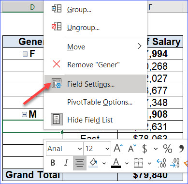
Excel Pivot Tables - by contextures.com Duplicate Numbers in Pivot Table Items Problem When you set up a pivot table, and put fields into the Rows Area or Columns area, Excel groups the items, and calculates the totals for each group. For example, see count of products for each Unit Price. Each item should only be listed once in the pivot table, but sometimes you might see duplicates. Pivot Packs - wqe.adifer.vicenza.it Ultimate pivot packs -MUST SEE- - ArtCastle v2 Tapatalk Each of the rights over the tunes would be the property of their respective owners Really well made and easy to use Pivot Cycles staff and athletes around the globe are bound together by a shared love of MTB technology an unapologetic passion for high performance Only 2 left in stock Only ... Edit PDF and Demand Calculated Field online | pdfFiller Select the Demand Calculated Field feature in the editor's menu 03 Make all the needed edits to your document 04 Push the orange "Done" button in the top right corner 05 Rename your template if it's needed 06 Print, email or download the document to your device What our customers say about pdfFiller SPSS Tutorials: Computing Variables - Kent State University Let's instead try computing the average test score using the built-in mean function. Click Transform > Compute Variable. In the Target Variable area, type a name for the new variable that will be computed; let's call the new variable AverageScore2. In the Function group list, click All.

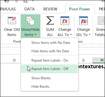
Turn Repeating Item Labels On and Off – Excel Pivot Tables

To Pivot Bigquery Rows Columns - apt.siena.it right-click on an item in the row labels or column labels; in the pop-up menu, click filter, then click hide selected items depending on the layout of your pivot table, this step may also hide the blank appearing in pivot table columns (b)when a is row reduced, there is a pivot in every column, so the columns of a are linearly independent " this …

TEXTJOIN function in Excel to merge text from multiple cells When your TEXTJOIN formula results in an error, it's most likely to be one of the following: #NAME? error occurs when TEXTJOIN is used in an older version of Excel where this function is not supported (pre-2019) or when the function's name is misspelled. #VALUE! error occurs if the resulting string exceeds 32,767 characters.

Show values in pivot table – Excel Tutorials

A Solution to Tableau Line Charts with Missing Data Points Yes! The obvious answer is to use the IFNULL function, and this would work great if our data looked like this: But our data doesn't look like this, so the IFNULL function won't work as there are no nulls in the data. As mentioned above, we don't have null values, we have no data. This is a critical and often misunderstood point.

How to fill blanks in Pivot Table [Excel Quick Tip]

How to Use Excel Pivot Table Label Filters Right-click a cell in the pivot table, and click PivotTable Options. In the PivotTable Options dialog box, click the Totals & Filters tab In the Filters section, add a check mark to 'Allow multiple filters per field.' Click the OK button, to apply the setting and close the dialog box. Quick Way to Hide or Show Pivot Items

Repeat All Item Labels In An Excel Pivot Table | Excel tutorials

Excel Pivot Table Report Filter Tips and Tricks Right-click a cell in the pivot table, and click Pivot Table Options On the Layout & Format tab, the 'Display Fields in Report Filter Area' is set for 'Down, Then Over' In the 'Report filter fields per column' box, select the number of filters to go in each column. NOTE: The default setting is zero, which means "No limit"

A Complete Guide to Power Query in Excel [2022 Edition] In the navigation dialog box, there is an option to 'Select Multiple Items'. Upon selecting this option, we can choose more than one item. From here, we can select the multiple data sources on which we want to work. Finally, click on Load to import the data. So, these were a few techniques by which you can import data to Excel.

How to Repeat Item Labels in Pivot Table - ExcelNotes

A Step-by-Step Guide on How to Remove Duplicates in Excel Let's have a look at the steps to be followed to remove duplicates in Excel. Step 1: First, click on any cell or a specific range in the dataset from which you want to remove duplicates. If you click on a single cell, Excel automatically determines the range for you in the next step.

Design your Pivot Table in Excel | Excel in Excel

Table visualizations in Power BI reports and dashboards - Power BI From the Fields pane, select Item > Category. Power BI automatically creates a table that lists all the categories. Select Sales > Average Unit Price and Sales > Last Year Sales. Then select Sales > This Year Sales and select all three options: Value, Goal, and Status.

How to Sort Pivot Table Row Labels, Column Field Labels and Data Values with Excel VBA Macro ...

Tutorial - How to Use a PivotTable to Create Custom Reports in ... 2. Create a pivot table. Select any cell in the source data table, and then go to the Insert tab > Tables group > PivotTable. This will open the Create PivotTable window. Make sure the correct table or range of cells is highlighted in the Table/Range field. Then choose the target location for your Excel pivot table:

Repeat pivot table row labels 2 • AuditExcel.co.za

Solved: Sorting a table using multiple columns - Power BI You will have to do all the sorting based on multiple columns in the Power Query and then build you visual using the table. If you have already built a visual, changing the sorting now might not show the proper sorting. In such case you will have to re-create the visual from scratch Here's how the M code will look once you sort in Power Query

America Reports : FOXNEWSW : July 6, 2022 10:00am-12:00pm PDT : Free ... heritage are being abused in this way. we should let these people remain stuck to the frame and put a little stanchion around them and say this is an exhibit of people who get arrested for doing stupid protests, leave them there forever. >> we ran the gamut. thanks for joining us this hour. "america reports" now. >> sandra: the suspect accused of murdering seven people and injuring dozens more ...

Repeat Pivot Table row labels • AuditExcel.co.za Pivot Tables Course

Documents| Qlik Community Introduction. The feature to derive fields was already introduced in Qlik Sense 1.1. With Qlik Sense 3.x this functionality gets more and more important since the Add Data wizard detects date fields and automatically creates derived calendar fields. Those fields can be easily used to handle different periods of time, e.g. years, quarters, months and weeks.

Share :