39 excel chart with labels from data
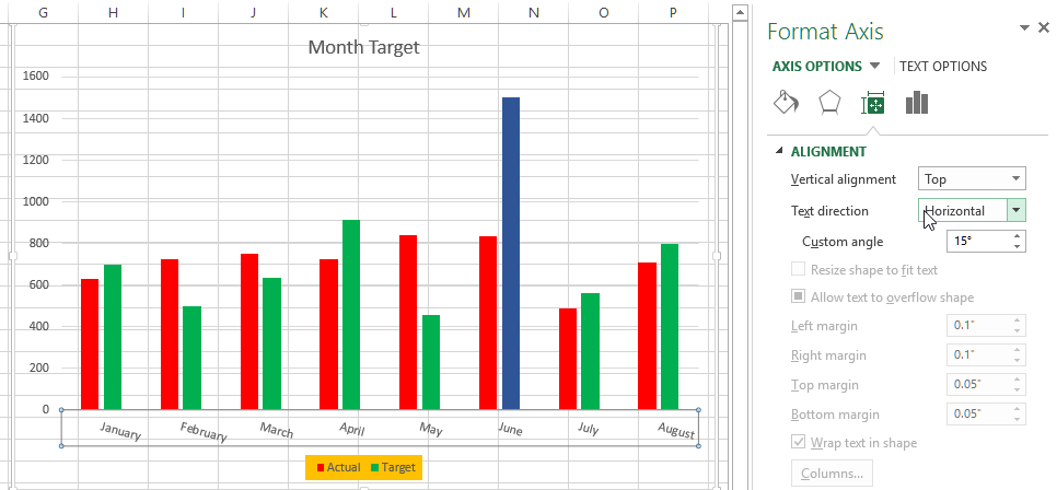
Custom Data Labels with Colors and Symbols in Excel Charts - [How To ... Step 4: Select the data in column C and hit Ctrl+1 to invoke format cell dialogue box. From left click custom and have your cursor in the type field and follow these steps: Press and Hold ALT key on the keyboard and on the Numpad hit 3 and 0 keys. Let go the ALT key and you will see that upward arrow is inserted. How to I rotate data labels on a column chart so that they are ... To change the text direction, first of all, please double click on the data label and make sure the data are selected (with a box surrounded like following image). Then on your right panel, the Format Data Labels panel should be opened. Go to Text Options > Text Box > Text direction > Rotate
How to Map Data in Excel (2 Easy Methods) - ExcelDemy For demonstration purposes, we are going to use the following dataset. Let's walk through the following steps. 📌 Steps: First of all, select the range of the dataset as shown below. Next, go to the Insert tab from your ribbon. Then, select Maps from the Tours group. Now, select the Open 3D Maps icon from the drop-down list
Excel chart with labels from data
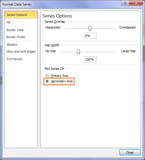
How to create Custom Data Labels in Excel Charts - Efficiency 365 Right click on any data label and choose the callout shape from Change Data Label Shapes option. Now adjust each data label as required to avoid overlap. Put solid fill color in the labels Finally, click on the chart (to deselect the currently selected label) and then click on a data label again (to select all data labels). How to Add Total Data Labels to the Excel Stacked Bar Chart Apr 03, 2013 · Step 4: Right click your new line chart and select “Add Data Labels” Step 5: Right click your new data labels and format them so that their label position is “Above”; also make the labels bold and increase the font size. Step 6: Right click the line, select “Format Data Series”; in the Line Color menu, select “No line” Step 7 ... Add / Move Data Labels in Charts - Excel & Google Sheets We'll start with the same dataset that we went over in Excel to review how to add and move data labels to charts. Add and Move Data Labels in Google Sheets Double Click Chart Select Customize under Chart Editor Select Series 4. Check Data Labels 5. Select which Position to move the data labels in comparison to the bars.
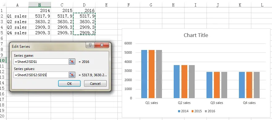
Excel chart with labels from data. Excel Chart Vertical Axis Text Labels • My Online Training Hub Apr 14, 2015 · So all we need to do is get that bar chart into our line chart, align the labels to the line chart and then hide the bars. We’ll do this with a dummy series: Copy cells G4:H10 (note row 5 is intentionally blank) > CTRL+C to copy the cells > select the chart > CTRL+V to paste the dummy data into the chart. How to Change Excel Chart Data Labels to Custom Values? - Chandoo.org May 05, 2010 · Now, click on any data label. This will select “all” data labels. Now click once again. At this point excel will select only one data label. Go to Formula bar, press = and point to the cell where the data label for that chart data point is defined. Repeat the process for all other data labels, one after another. See the screencast. Add or remove data labels in a chart - support.microsoft.com Data labels make a chart easier to understand because they show details about a data series or its individual data points. For example, in the pie chart below, without the data labels it would be difficult to tell that coffee was 38% of total sales. ... You can add data labels to show the data point values from the Excel sheet in the chart ... Creating a chart with dynamic labels - Microsoft Excel 2016 1. Right-click on the chart and in the popup menu, select Add Data Labels and again Add Data Labels : 2. Do one of the following: For all labels: on the Format Data Labels pane, in the Label Options, in the Label Contains group, check Value From Cells and then choose cells: For the specific label: double-click on the label value, in the popup ...
How to Insert Axis Labels In An Excel Chart | Excelchat The method below works in the same way in all versions of Excel. How to add horizontal axis labels in Excel 2016/2013 . We have a sample chart as shown below; Figure 2 – Adding Excel axis labels. Next, we will click on the chart to turn on the Chart Design tab; We will go to Chart Design and select Add Chart Element; Figure 3 – How to label ... How to Create Charts in Excel (In Easy Steps) - Excel Easy 1. Select the chart. 2. On the Chart Design tab, in the Type group, click Change Chart Type. 3. On the left side, click Column. 4. Click OK. Result: Switch Row/Column If you want to display the animals (instead of the months) on the horizontal axis, execute the following steps. 1. Select the chart. 2. Excel Charts - Aesthetic Data Labels - tutorialspoint.com To place the data labels in the chart, follow the steps given below. Step 1 − Click the chart and then click chart elements. Step 2 − Select Data Labels. Click to see the options available for placing the data labels. Step 3 − Click Center to place the data labels at the center of the bubbles. Format a Single Data Label How to Place Labels Directly Through Your Line Graph in Microsoft Excel ... Right-click on top of one of those circular data points. You'll see a pop-up window. Click on Add Data Labels. Your unformatted labels will appear to the right of each data point: Click just once on any of those data labels. You'll see little squares around each data point. Then, right-click on any of those data labels. You'll see a pop-up menu.
How to add data labels from different column in an Excel chart? This method will guide you to manually add a data label from a cell of different column at a time in an Excel chart. 1.Right click the data series in the chart, and select Add Data Labels > Add Data Labels from the context menu to add data labels.. 2. Show numbers in thousands in Excel as K in table or chart Show in thousands (K) or millions (M) on the Excel chart axis. If you want to show numbers in thousands or millions on the Excel chart axis, change the axis display units options. Format axis (select axis labels, and press Ctrl + 1) and change display units like this. As the result, you will get something like this. Example: Charts with Data Labels — XlsxWriter Documentation A demo of some of the Excel chart data labels options that are available via an XlsxWriter chart. These include custom labels with user text or text taken from cells in the worksheet. See also Chart series option: Data Labels and Chart series option: Custom Data Labels. Chart 1 in the following example is a chart with standard data labels: Change the format of data labels in a chart To get there, after adding your data labels, select the data label to format, and then click Chart Elements > Data Labels > More Options. To go to the appropriate area, click one of the four icons ( Fill & Line, Effects, Size & Properties ( Layout & Properties in Outlook or Word), or Label Options) shown here.
Excel Custom Chart Labels • My Online Training Hub
How to Use Cell Values for Excel Chart Labels - How-To Geek Select the chart, choose the "Chart Elements" option, click the "Data Labels" arrow, and then "More Options." Uncheck the "Value" box and check the "Value From Cells" box. Select cells C2:C6 to use for the data label range and then click the "OK" button. The values from these cells are now used for the chart data labels.

How to edit the label of a chart in Excel? - Stack Overflow
Add or remove data labels in a chart - support.microsoft.com Click the data series or chart. To label one data point, after clicking the series, click that data point. In the upper right corner, next to the chart, click Add Chart Element > Data Labels. To change the location, click the arrow, and choose an option. If you want to show your data label inside a text bubble shape, click Data Callout.
Add Average Marker to Excel Box Plot - Box and Whisker Chart - YouTube
HOW TO CREATE A BAR CHART WITH LABELS INSIDE BARS IN EXCEL - simplexCT 7. In the chart, right-click the Series "# Footballers" Data Labels and then, on the short-cut menu, click Format Data Labels. 8. In the Format Data Labels pane, under Label Options selected, set the Label Position to Inside End. 9. Next, in the chart, select the Series 2 Data Labels and then set the Label Position to Inside Base.
How-to Use Data Labels from a Range in an Excel Chart - Excel Dashboard Templates
Add data labels and callouts to charts in Excel 365 - EasyTweaks.com Step #1: After generating the chart in Excel, right-click anywhere within the chart and select Add labels . Note that you can also select the very handy option of Adding data Callouts. Step #2: When you select the "Add Labels" option, all the different portions of the chart will automatically take on the corresponding values in the table ...
30 How To Label A Chart In Excel - Labels Niche Ideas
How To Add Data Labels In Excel ~ Pvkngcchittoor Then, click the insert tab along the top ribbon and click the insert scatter (x,y) option in the charts group. Click on the arrow next to data labels to change the position of where the labels are in relation to the bar chart. To format data labels in excel, choose the set of data labels to format. Source:
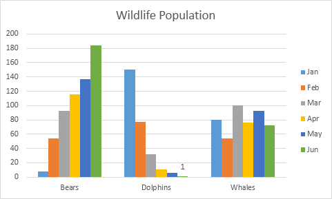
Excel clustered column chart - Access-Excel.Tips
Custom Chart Data Labels In Excel With Formulas - How To Excel At Excel Follow the steps below to create the custom data labels. Select the chart label you want to change. In the formula-bar hit = (equals), select the cell reference containing your chart label's data. In this case, the first label is in cell E2. Finally, repeat for all your chart laebls.
Charts and Graphs in Excel
Excel: How to Create a Bubble Chart with Labels - Statology Step 3: Add Labels. To add labels to the bubble chart, click anywhere on the chart and then click the green plus "+" sign in the top right corner. Then click the arrow next to Data Labels and then click More Options in the dropdown menu: In the panel that appears on the right side of the screen, check the box next to Value From Cells within ...
Create a Chart in Excel - Tech Funda
How to group (two-level) axis labels in a chart in Excel? - ExtendOffice The Pivot Chart tool is so powerful that it can help you to create a chart with one kind of labels grouped by another kind of labels in a two-lever axis easily in Excel. You can do as follows: 1. Create a Pivot Chart with selecting the source data, and: (1) In Excel 2007 and 2010, clicking the PivotTable > PivotChart in the Tables group on the ...

Multiple Series in One Excel Chart - Peltier Tech Blog
How To Use Dynamic Data Labels To Create Interactive Excel Charts Insert An Interactive Line Chart With Dynamic Data Labels. Select the data and insert a combo chart. For combo, chart go to the Insert → Charts → Combo Charts. Now make a selection for the Line Chart for revenue data and a Line Chart With Markers For Data Labels. Now select the Data Label Line and remove fill color from it.

MRP Template and Calculator for Excel
How to Add Labels to Scatterplot Points in Excel - Statology Next, click anywhere on the chart until a green plus (+) sign appears in the top right corner. Then click Data Labels, then click More Options… In the Format Data Labels window that appears on the right of the screen, uncheck the box next to Y Value and check the box next to Value From Cells.
Excel Gantt Chart - Free Excel Templates
Data Labels in Excel Pivot Chart (Detailed Analysis) 7 Suitable Examples with Data Labels in Excel Pivot Chart Considering All Factors 1. Adding Data Labels in Pivot Chart 2. Set Cell Values as Data Labels 3. Showing Percentages as Data Labels 4. Changing Appearance of Pivot Chart Labels 5. Changing Background of Data Labels 6. Dynamic Pivot Chart Data Labels with Slicers 7.
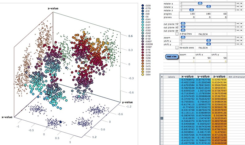
3d scatter plot for MS Excel
How to add data labels from different column in an Excel chart? Right click the data series in the chart, and select Add Data Labels > Add Data Labels from the context menu to add data labels. 2. Click any data label to select all data labels, and then click the specified data label to select it only in the chart. 3.
Quickly create a progress bar with percentage in Excel
Excel tutorial: How to use data labels Generally, the easiest way to show data labels to use the chart elements menu. When you check the box, you'll see data labels appear in the chart. If you have more than one data series, you can select a series first, then turn on data labels for that series only. You can even select a single bar, and show just one data label.

Enable or Disable Excel Data Labels at the click of a button - How To - PakAccountants.com
How to create a chart with both percentage and value in Excel? In the Format Data Labels pane, please check Category Name option, and uncheck Value option from the Label Options, and then, you will get all percentages and values are displayed in the chart, see screenshot: 15.

How to edit the label of a chart in Excel? - Stack Overflow
Create Dynamic Chart Data Labels with Slicers - Excel Campus Feb 10, 2016 · Typically a chart will display data labels based on the underlying source data for the chart. In Excel 2013 a new feature called “Value from Cells” was introduced. This feature allows us to specify the a range that we want to use for the labels. Since our data labels will change between a currency ($) and percentage (%) formats, we need a ...

E-xcel Tuts: Add Data Labels to Excel Charts
Adding rich data labels to charts in Excel 2013 | Microsoft 365 Blog Putting a data label into a shape can add another type of visual emphasis. To add a data label in a shape, select the data point of interest, then right-click it to pull up the context menu. Click Add Data Label, then click Add Data Callout . The result is that your data label will appear in a graphical callout.
How to Add Data Labels in an Excel Chart in Excel 2010 - YouTube
How to Print Labels from Excel - Lifewire Select Mailings > Write & Insert Fields > Update Labels . Once you have the Excel spreadsheet and the Word document set up, you can merge the information and print your labels. Click Finish & Merge in the Finish group on the Mailings tab. Click Edit Individual Documents to preview how your printed labels will appear. Select All > OK .
Post a Comment for "39 excel chart with labels from data"