39 value data labels excel

Custom Chart Data Labels In Excel With Formulas - How To Excel At Excel Follow the steps below to create the custom data labels. Select the chart label you want to change. In the formula-bar hit = (equals), select the cell reference containing your chart label's data. In this case, the first label is in cell E2. Finally, repeat for all your chart laebls. DataLabels.ShowValue property (Excel) | Microsoft Learn Example. This example enables the value to be shown for the data labels of the first series, on the first chart. This example assumes that a chart exists on the active worksheet. VB. Sub UseValue () ActiveSheet.ChartObjects (1).Activate ActiveChart.SeriesCollection (1) _ .DataLabels.ShowValue = True End Sub.

Multiple data labels (in separate locations on chart) Re: Multiple data labels (in separate locations on chart) You can do it in a single chart. Create the chart so it has 2 columns of data. At first only the 1 column of data will be displayed. Move that series to the secondary axis. You can now apply different data labels to each series. Attached Files 819208.xlsx‎ (13.8 KB, 267 views) Download

Value data labels excel

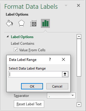
Add a DATA LABEL to ONE POINT on a chart in Excel Steps shown in the video above: Click on the chart line to add the data point to. All the data points will be highlighted. Click again on the single point that you want to add a data label to. Right-click and select ' Add data label ' This is the key step! Right-click again on the data point itself (not the label) and select ' Format data label '. [CELLRANGE] instead of value on graph? - Microsoft Community This happens when the chart data labels come from a range of cells and have been added with the feature "Value from cells" in Excel 2013 or higher. This feature will show as "Cellrange" in older versions of Excel. This screenshot shows how you can use "Value from cells" to select a range of cells for data labels in a chart in Excel 2013. Data Label Values from Cells - Microsoft Community Hub Click on one of the bars in the chart to display the formula for the chart. It will look like SERIES (,,'tester'!$D$23:$J$23,1). Change it to = SERIES (,,trial.xlsx!tribe,1) That is using the name of the spreadsheet, not the worksheet, and the name of the range created in the name manager.

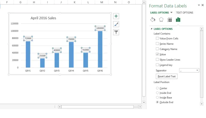
Value data labels excel. › documents › excelHow to hide zero data labels in chart in Excel? - ExtendOffice Sometimes, you may add data labels in chart for making the data value more clearly and directly in Excel. But in some cases, there are zero data labels in the chart, and you may want to hide these zero data labels. Here I will tell you a quick way to hide the zero data labels in Excel at once. Hide zero data labels in chart Excel Data Labels - Value from Cells When I recheck the data labels, Format Data Labels, "Value from Cells" is still checked and the cell range is still correct and includes the cell with the new label. I can select "Reset Label Text", uncheck "Value from Cells" re-check and then it appears. I Save and Close. The issue reappears for the next new data point. Format Data Labels in Excel- Instructions - TeachUcomp, Inc. To format data labels in Excel, choose the set of data labels to format. To do this, click the "Format" tab within the "Chart Tools" contextual tab in the Ribbon. Then select the data labels to format from the "Chart Elements" drop-down in the "Current Selection" button group. Change the format of data labels in a chart To get there, after adding your data labels, select the data label to format, and then click Chart Elements > Data Labels > More Options. To go to the appropriate area, click one of the four icons ( Fill & Line, Effects, Size & Properties ( Layout & Properties in Outlook or Word), or Label Options) shown here.

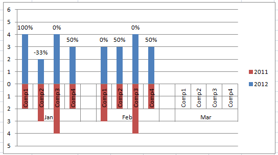
Excel, giving data labels to only the top/bottom X% values But even if a cell is visually blank, Excel's charting functions interprets the value as 0 if there is a formula in the cell. This means the entire bottom of the graph has repeated data labels of "0%". To solve this I set the value of the FALSE parameter as a negative number and then changed the minimum value on the graph from automatic to 0. › publication › 344638517_Excel(PDF) Excel For Statistical Data Analysis - ResearchGate Oct 14, 2020 · This site provides illustrative experience in the use of Excel for data summary, presentation, ... that value) then select Labels. Enter 0.05 or, whatever level of signiﬁcance you desire, ... realpython.com › pandas-dataframeThe Pandas DataFrame: Make Working With Data Delightful .at[] accepts the labels of rows and columns and returns a single data value..iat[] accepts the zero-based indices of rows and columns and returns a single data value. Of these, .loc[] and .iloc[] are particularly powerful. They support slicing and NumPy-style indexing. You can use them to access a column: >>> Excel tutorial: Dynamic min and max data labels To make the formula easy to read and enter, I'll name the sales numbers "amounts". The formula I need is: =IF (C5=MAX (amounts), C5,"") When I copy this formula down the column, only the maximum value is returned. And back in the chart, we now have a data label that shows maximum value. Now I need to extend the formula to handle the minimum value.

support.microsoft.com › en-us › officeUsing Access or Excel to manage your data User-level data protection In Excel, you can remove critical or private data from view by hiding columns and rows of data, and then protect the whole worksheet to control user access to the hidden data. In addition to protecting a worksheet and its elements, you can also lock and unlock cells in a worksheet to prevent other users from ... How to Add Data Labels to an Excel 2010 Chart - dummies On the Chart Tools Layout tab, click Data Labels→More Data Label Options. The Format Data Labels dialog box appears. You can use the options on the Label Options, Number, Fill, Border Color, Border Styles, Shadow, Glow and Soft Edges, 3-D Format, and Alignment tabs to customize the appearance and position of the data labels. › how-to-select-best-excelBest Types of Charts in Excel for Data Analysis, Presentation ... Apr 29, 2022 · Learn to select the best types of Charts in Excel for Data Analysis, Presentation and Reporting. Get the FREE ebook on "Best Excel Charts" (40 pages) DataLabel object (Excel) | Microsoft Learn Use DataLabels ( index ), where index is the data-label index number, to return a single DataLabel object. The following example sets the number format for the fifth data label in series one in embedded chart one on worksheet one. VB Worksheets (1).ChartObjects (1).Chart _ .SeriesCollection (1).DataLabels (5).NumberFormat = "0.000"

How To Show Or Hide Data Labels On MS Excel? | My Windows Hub

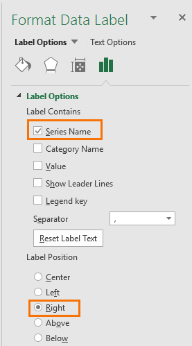
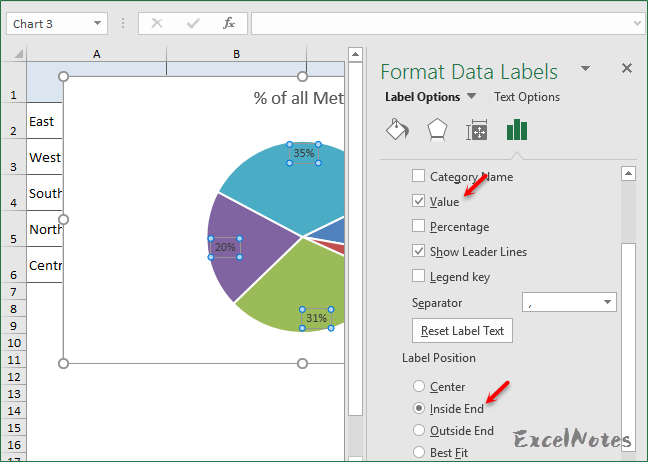
How to Add Two Data Labels in Excel Chart (with Easy Steps) You can easily show two parameters in the data label. For instance, you can show the number of units as well as categories in the data label. To do so, Select the data labels. Then right-click your mouse to bring the menu. Format Data Labels side-bar will appear. You will see many options available there. Check Category Name.

How to Add Data Labels to an Excel 2010 Chart - dummies

How to Add Data Labels in Excel - Excelchat | Excelchat In Excel 2013 and the later versions we need to do the followings; Click anywhere in the chart area to display the Chart Elements button Figure 5. Chart Elements Button Click the Chart Elements button > Select the Data Labels, then click the Arrow to choose the data labels position. Figure 6. How to Add Data Labels in Excel 2013 Figure 7.

Adding rich data labels to charts in Excel 2013 | Microsoft ...

› excel_data_analysis › excelExcel Data Analysis - Data Visualization - tutorialspoint.com Data Labels. Excel 2013 and later versions provide you with various options to display Data Labels. You can choose one Data Label, format it as you like, and then use Clone Current Label to copy the formatting to the rest of the Data Labels in the chart. The Data Labels in a chart can have effects, varying shapes and sizes.

Format Number Options for Chart Data Labels in PowerPoint ...

How to Add Total Data Labels to the Excel Stacked Bar Chart Step 4: Right click your new line chart and select "Add Data Labels" Step 5: Right click your new data labels and format them so that their label position is "Above"; also make the labels bold and increase the font size. Step 6: Right click the line, select "Format Data Series"; in the Line Color menu, select "No line"

Add or remove data labels in a chart

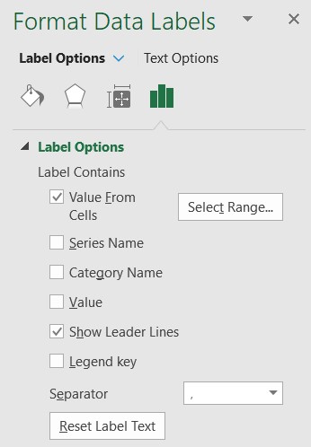
How to add data labels from different column in an Excel chart? In the Format Data Labels pane, under Label Options tab, check the Value From Cells option, select the specified column in the popping out dialog, and click the OK button. Now the cell values are added before original data labels in bulk. 4. Go ahead to untick the Y Value option (under the Label Options tab) in the Format Data Labels pane.

Format Number Options for Chart Data Labels in Excel 2011 for Mac

How to show data label in "percentage" instead of "value" in stacked ... Select Format Data Labels Select Number in the left column Select Percentage in the popup options In the Format code field set the number of decimal places required and click Add. (Or if the table data in in percentage format then you can select Link to source.) Click OK Regards, OssieMac Report abuse 8 people found this reply helpful ·

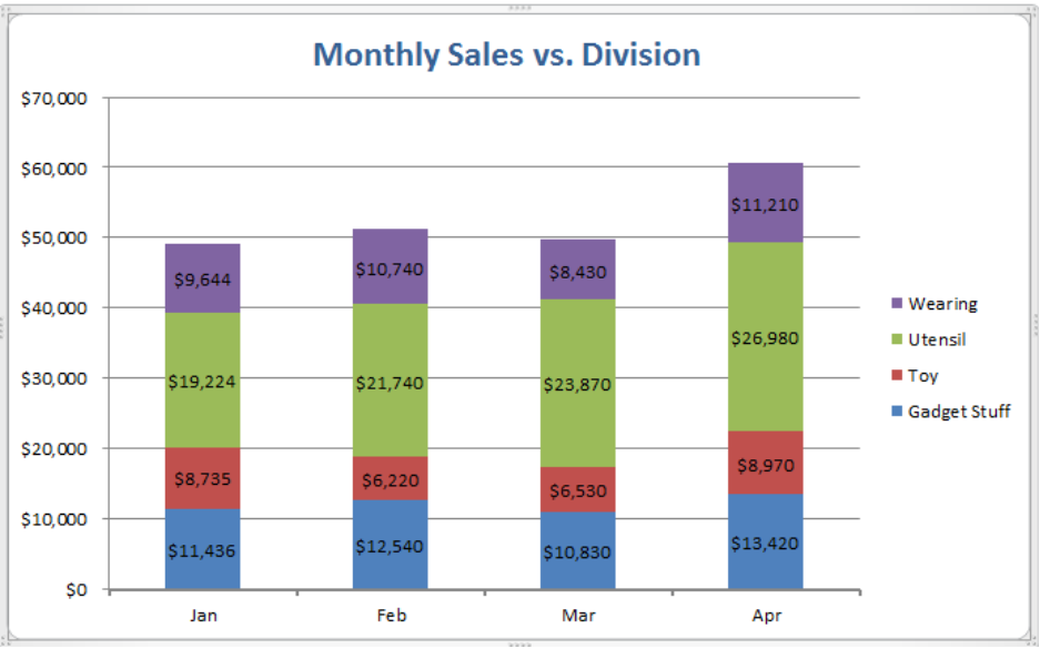
Add Total Values for Stacked Column and Stacked Bar Charts in ...

techcommunity.microsoft.com › t5 › azure-dataDirect Query from Excel to Azure Data Explorer (aka Kusto) Dec 08, 2021 · You can also add the data to the Excel data model and add more data from other sources. After we select our parameter values, we can click on refresh all and the pivot will be refreshed based on the values selected in Excel . Building the report . Bringing the list of Event Types . Our first query will bring the list of Event Types from the table.

Custom data labels in a chart

Excel- Labels, Values, and Formulas - WebJunction Excel Labels, Values, and Formulas. Labels and values. Entering data into a spreadsheet is just like typing in a word processing program, but you have to first click the cell in which you want the data to be placed before typing the data. All words describing the values (numbers) are called labels.

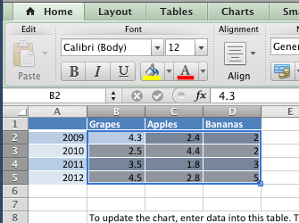
How to Use Cell Values for Excel Chart Labels

what happened to "value from cells"? - Microsoft Community Hub what happened to "value from cells"? In a chart: Data labels, more options, format data labels, label options, label contains value from cells Usually it the option is there, today, sometimes/mostly, it is not. These are x-y scatter graphs.

How to add data labels from different column in an Excel chart?

How to Change Excel Chart Data Labels to Custom Values? - Chandoo.org Define the new data label values in a bunch of cells, like this: Now, click on any data label. This will select "all" data labels. Now click once again. At this point excel will select only one data label. Go to Formula bar, press = and point to the cell where the data label for that chart data point is defined.

How to add or move data labels in Excel chart?

Custom Data Labels with Colors and Symbols in Excel Charts - [How To ... To apply custom format on data labels inside charts via custom number formatting, the data labels must be based on values. You have several options like series name, value from cells, category name. But it has to be values otherwise colors won't appear. Symbols issue is quite beyond me.

Adding rich data labels to charts in Excel 2013 | Microsoft ...

Add or remove data labels in a chart - support.microsoft.com Click Label Options and under Label Contains, pick the options you want. Use cell values as data labels You can use cell values as data labels for your chart. Right-click the data series or data label to display more data for, and then click Format Data Labels. Click Label Options and under Label Contains, select the Values From Cells checkbox.

How to hide zero data labels in chart in Excel?

How to Use Cell Values for Excel Chart Labels - How-To Geek Select the chart, choose the "Chart Elements" option, click the "Data Labels" arrow, and then "More Options." Uncheck the "Value" box and check the "Value From Cells" box. Select cells C2:C6 to use for the data label range and then click the "OK" button. The values from these cells are now used for the chart data labels.

How-to Use Data Labels from a Range in an Excel Chart - Excel ...

Adding rich data labels to charts in Excel 2013 Then, select the value in the data label and hit the right-arrow key on your keyboard. The story behind the data in our example is that the temperature increased significantly on Wednesday and that appeared to help drive up business at the lemonade stand. So I type some text to emphasize that point while still leaving the data label intact.

Custom Data Labels with Colors and Symbols in Excel Charts ...

Data Labels in Excel Pivot Chart (Detailed Analysis) 7 Suitable Examples with Data Labels in Excel Pivot Chart Considering All Factors 1. Adding Data Labels in Pivot Chart 2. Set Cell Values as Data Labels 3. Showing Percentages as Data Labels 4. Changing Appearance of Pivot Chart Labels 5. Changing Background of Data Labels 6. Dynamic Pivot Chart Data Labels with Slicers 7.

How to add live total labels to graphs and charts in Excel ...

Series.DataLabels method (Excel) | Microsoft Learn Return value. Object. Remarks. If the series has the Show Value option turned on for the data labels, the returned collection can contain up to one label for each point. Data labels can be turned on or off for individual points in the series. If the series is on an area chart and has the Show Label option turned on for the data labels, the returned collection contains only a single label ...

Custom Chart Data Labels In Excel With Formulas

Data Label Values from Cells - Microsoft Community Hub Click on one of the bars in the chart to display the formula for the chart. It will look like SERIES (,,'tester'!$D$23:$J$23,1). Change it to = SERIES (,,trial.xlsx!tribe,1) That is using the name of the spreadsheet, not the worksheet, and the name of the range created in the name manager.

Adding rich data labels to charts in Excel 2013 | Microsoft ...

[CELLRANGE] instead of value on graph? - Microsoft Community This happens when the chart data labels come from a range of cells and have been added with the feature "Value from cells" in Excel 2013 or higher. This feature will show as "Cellrange" in older versions of Excel. This screenshot shows how you can use "Value from cells" to select a range of cells for data labels in a chart in Excel 2013.